Originally posted on: https://medium.com/@steinsfu/stylegan3-clearly-explained-793edbcc8048

Paper Explained: StyleGAN3 — Alias-Free Generative Adversarial Networks

The StyleGAN3 paper is pretty hard to understand. In this article, I tried my best to reorganize it and explain it step by step.

Hope you understand it better after reading this.

If you want to know the difference and evolution of StyleGAN, StyleGAN2, StyleGAN2-ADA, and StyleGAN3, you can read the following article.

StyleGAN vs StyleGAN2 vs StyleGAN2-ADA vs StyleGAN3

In this article, I will compare and show you the evolution of StyleGAN, StyleGAN2, StyleGAN2-ADA, and StyleGAN3.

medium.com

Table of Contents

• Introduction
• Texture Sticking Problem
• Reason: Positional References
• Goal
• Discrete vs Continuous Domain
• Redesigning Network Layers
• Changes
• Results
• References

Introduction

The purpose of StyleGAN3 is to tackle the “texture sticking” issue that happened in the morphing transition (e.g. morphing from one face to another face) in StyleGAN2.

In other words, StyleGAN3 tries to make the transition animation more natural.

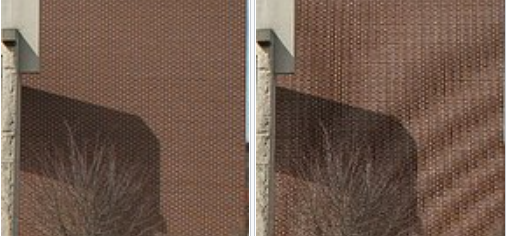
Texture Sticking Problem

As you can see from the above animations, the beard and hair (left) look like sticking to the screen when morphing, while the one generated by StyleGAN3 (right) does not have this sticky pixels problem.

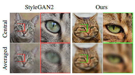
The average of images is sharp in StyleGAN2 as many details (e.g. fur) stick to the same pixel coordinates, while the intended result should be uniformly blurry because all details should move together when morphing.

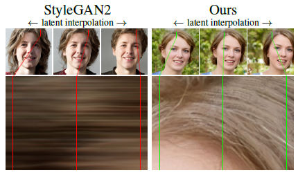
Again, the desired result is hairs moving in animation (right), but not sticking to the same coordinates (left).

Reason: Positional References

It turns out that there are some unintentional positional references available in the intermediate layers for the network to process feature maps through the following sources:

• Image borders
• Per-pixel noise inputs
• Positional encodings
• Aliasing

These positional references make the network generates pixels sticking to the same coordinates.

Among them, aliasing is the hardest one to identify and fix.

Aliasing

Aliasing is an effect that causes different signals to become indistinguishable (or aliases of one another) when sampled.

It also often refers to the distortion or artifact that results when a signal reconstructed from samples is different from the original continuous signal.

E.g. When we sample a high-frequency signal (e.g. the blue sine wave), if it results in a lower frequency signal (the red wave), then this is called aliasing since it is completely different from the original signal. This happens because the sampling rate is too low.

The researchers have identified two sources for aliasing in GAN:

1. Faint after-images of the pixel grid resulting from non-ideal upsampling filters (e.g. nearest, bilinear, or stridden convolutions)
2. The pointwise application of nonlinearities (e.g. ReLU, or swish)

Even with a small amount of aliasing, it is amplified throughout the network and becomes a fixed position in the screen coordinates.

Goal

The goal is to eliminate all sources of positional references. After that, the details of the images can be generated equally well regardless of pixel coordinates.

In order to remove positional references, the paper proposed to make the network equivariant:

Consider an operation f (e.g. convolution, upsampling, ReLU, etc.) and a spatial transformation t (e.g. translation, rotation).

f is equivariant with respect to t if t ○ f = f ○ t.

In other words, an operation (e.g. ReLU), should not insert any positional codes/references which will affect the transformation procedure, and vice versa.

Limitation of Discrete Domain

However, this is very hard to achieve in traditional neural network layers, because they operate in the discrete domain (e.g. pixels).

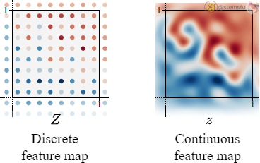
These discrete feature maps can be regarded as the sampling results from their underlying continuous feature maps (which are just imaginary because they don’t really exist. We can imagine it as the discrete feature map becoming infinitely high-resolution, like a continuous signal).

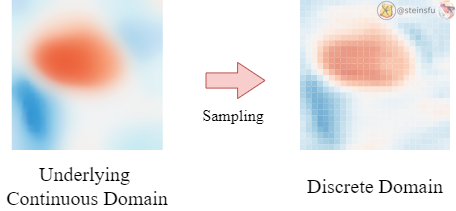
So, it turns out that the whole traditional network is operating on these unfaithful sampled discrete feature maps and hence introducing severe aliasing over the network.

Switch to Continuous Domain

Therefore, we would like to switch all the operations in the network from the discrete domain to the continuous domain. To achieve this, we have to redesign all the operation layers:

• Convolution
• Upsampling/Downsampling
• Nonlinearity (e.g. ReLU)

Discrete vs Continuous Domain

Now, we know that traditional neural networks operate on discretely sampled feature maps.

Before we talk about how we redesign the network layers, let’s take a look at how we convert between discrete and continuous signals.

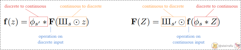
Conversion Between Discrete and Continuous

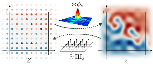
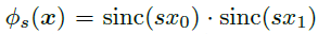
Φₛ: a low-pass filter, which is used to remove the problematic frequencies that will cause aliasing.

IIIₛ: an infinite series of Dirac delta functions spaced at even intervals. Applying Dirac comb on z simply means to sample from z and get the discretized feature map Z.

Continuous to Discrete

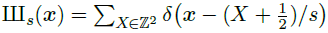
Converting a continuous signal to a discrete signal is fairly simple. We just need to sample from z using the Dirac comb IIIₛ. Where ⊙ denotes pointwise multiplication.

Discrete to Continuous

Converting a discrete signal to a continuous signal is a bit complicated.

The Whittaker-Shannon interpolation formula states that the corresponding continuous representation z is obtained by convolving the discretely sampled Dirac grid Z with an ideal interpolation (low-pass) filter Φₛ, where s is the sampling rate.

i.e. z(x) = (Φₛ * Z)(x), where * denotes the continuous convolution.

Before explaining the low-pass filter, let’s see how a continuous signal can be decomposed into different frequencies sine waves.

Decomposing Signals

A complicated continuous signal is actually a mixture of multiple sinusoids. We can decompose it using Fourier Transform to unveil these sine waves of different frequencies.

Low-pass filter

A low-pass filter is a filter that allows low-frequency signals (i.e. of these decomposed sinusoids) to pass, and attenuates (weakens) high-frequency signals or even stops them from passing.

Convolution with Low-pass Filter

By convolving the discrete Dirac grid Z using the low-pass filter Φₛ, we can convert the discrete signal Z to the continuous signal z.

Sampling Rate

According to the Nyquist-Shannon sampling theorem, if the sampling rate = s, all frequencies less than s/2 will not alias.

Since Φₛ has a band limit of s/2 along the horizontal and vertical dimensions, it ensures that the resulting continuous signal captures all frequencies that can be represented with sampling rate s.

Redesigning Network Layers

Practical neural networks operate on discretely sampled feature maps.

Let’s denote F as an operation (e.g. convolution, upsampling/downsampling, nonlinearity, etc.) operating on a discrete feature map Z: Z’ = F(Z).

There will also be a corresponding continuous counterpart feature map z, so we have a corresponding mapping f in the continuous domain: z’ = f(z).

So, an operation specified in one domain can be seen to perform a corresponding operation in the other domain:

Convolution Layer

Consider a standard convolution with a discrete kernel K and a sampling rate s. The discrete domain convolution is simply F_conv(Z)=K*Z. We can obtain the continuous domain convolution from Eq.1.

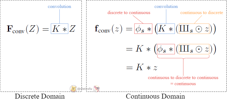
It turns out that the convolution operates by continuously sliding the discretized kernel K over the continuous representation of the feature map z.

This convolution introduces no new frequencies, so the bandlimit requirements for both translation and rotation equivariance are trivially fulfilled.

(Note: if the operation introduces new frequencies, the sampling rate of the low-pass filter might need to be adjusted such that the highest frequency < s/2 to avoid aliasing)

Upsampling

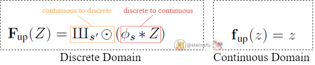
Ideal upsampling does not modify the continuous representation (i.e. f_up(z)=z), because a continuous signal already has the finest detail. Therefore, the translation and rotation equivariance are directly fulfilled in the continuous domain.

We can then obtain the discrete domain upsampling from Eq.1. By choosing s’=ns, where n is an integer, we can upsample the feature map with a factor of n (e.g. n=2 means upsampling the feature map 2 times bigger in each dimension).

Downsampling

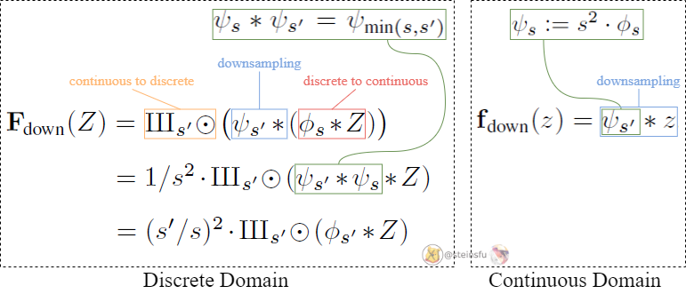
In the continuous domain, ψₛ:= s² · Φₛ is simply the interpolation filter normalized to unit mass. It acts as a low-pass filter to remove frequencies above the output band limit (to avoid aliasing) so that the signal can be represented faithfully in the coarser discretization.

We can then obtain the discrete domain downsampling from Eq.1. Similar to upsampling, downsampling by an integer fraction can be implemented with a discrete convolution followed by dropping sample points, i.e. ns’=s.

Translation equivariance follows automatically from the commutativity of f_down(z) with translation. However, for rotation equivariance, we must replace Φₛ’ with a radially symmetric filter with disc-shaped frequency response.

Nonlinearity

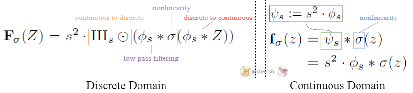
Nonlinearity layers such as ReLU in the continuous domain may introduce arbitrarily high frequencies that cannot be represented in the output (aliasing).

The solution is to eliminate the offending high-frequency content by convolving the continuous result with the ideal low-pass filter ψₛ:= s² · Φₛ. Then, we have our continuous domain nonlinearity function.

In the continuous domain, any pointwise function commutes trivially with translation and rotation (equivariance).

We can then obtain the discrete domain nonlinearity from Eq.1.

In the discrete domain, we have found that only a 2× temporary resolution increase is sufficient for high-quality equivariance. For rotation equivariance, we must use the radially symmetric interpolation filter in the downsampling step.

The above diagram is the visualization of filtered nonlinearity.

• Top row: the continuous signals
• Middle row: sampled from the continuous signal
• Bottom row: reconstructed from the discretized signal

Left column: z is the ideal signal. As the sampling rate is high enough to capture the signal, no aliasing occurs.

Middle column: σ(z) means applying a pointwise nonlinearity (e.g. ReLU) to z. As the high frequencies created by the clipping cannot be represented by the sample grid, aliasing occurs.

Right column: Applying a low-pass filter to the nonlinearity leads to a faithful reconstruction, no aliasing occurs.

Changes

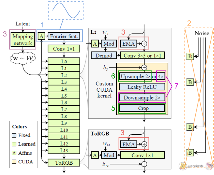
1. Replaced the learned input constant in StyleGAN2 with Fourier feature to facilitate exact continuous translation and rotation of z.
2. Removed the per-pixel noise inputs to eliminate positional references introduced by them.
3. Decreased the mapping network depth to simplify the setup.
4. Eliminated the output skip connections (which were used to deal with the gradient vanishing problem. We address that by using a simple normalization before each convolution, i.e. divided by EMA: Exponential Moving Average)
5. Maintained a fixed-size margin around the target canvas, cropping to this extended canvas after each layer (to leak absolute image coordinates into internal representations, because the signals outside the canvas are also important).
6. Replaced the bilinear 2× upsampling filter with a better approximation of the ideal low-pass filter.
7. Motivated by our theoretical model, we wrap the leaky ReLU between m×upsampling and m×downsampling. (we can fuse the previous 2×upsampling with this m×upsampling, i.e. choose m=2, then we have 4×upsampling before each leaky ReLU)

Translation Equivariance (Config T)

In a previous config (config G), we set the cutoff frequency to f_c = s/2-f_h, which ensures that all alias frequencies (above s/2) are in the stopband (a.k.a are removed) in order to suppress aliasing.

In config G, we chose to lower f_c on all layers except the highest-resolution ones, because in the end the generator must be able to produce crisp (detailed/sharp) images to match the training data.

Our changes have improved the equivariance quality considerably, but some visible artifacts still remain. To further suppress aliasing, we need stronger attenuation in the lowest-resolution layers.

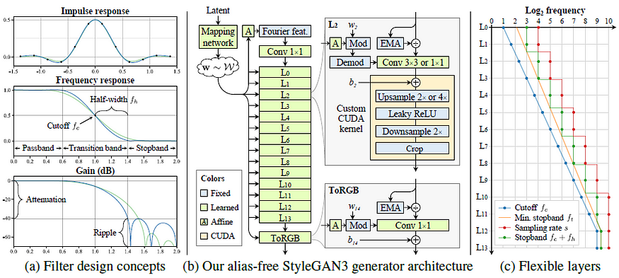
In particular, we would like f_h to be high in the lowest-resolution layers to maximize attenuation in the stopband, but low in the highest-resolution layers to allow matching high-frequency details of the training data.

Remind that f_c = s/2-f_h.

This progressively decreasing of f_h improve translation equivariance, eliminating the remaining artifacts.

Rotation Equivariance (Config R)

We obtain a rotation equivariance version of the network with two changes:

1. Replacing the 3×3 convolutions with 1×1 on all layers and compensating for the reduced capacity by doubling the number of feature maps.
2. Replacing the sinc-based downsampling filter with a radially symmetric jinc-based filter.

Results

The alias-free translation (middle) and rotation (bottom) equivariant networks build the image in a radically different manner from what appear to be multi-scale phase signals that follow the features seen in the final image.

In the internal representations, it looks like a new coordinate system is being invented and details are drawn on these surfaces.

References

[1] T. Karras et al., “Alias-Free Generative Adversarial Networks”, arXiv.org, 2022. https://arxiv.org/abs/2106.12423

[2] “Aliasing — Wikipedia”, En.wikipedia.org, 2022. https://en.wikipedia.org/wiki/Aliasing

[3] J. Wang et al., “CNN Explainer”, Poloclub.github.io, 2022. https://poloclub.github.io/cnn-explainer

[4] “Fourier transform — Wikipedia”, En.wikipedia.org, 2022. https://en.wikipedia.org/wiki/Fourier_transform